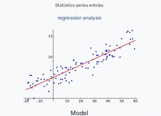
Multiple linear regression is a widely used regression analysis method in statistics and machine learning. By analyzing the relationship between multiple independent variables and a dependent variable, it helps us understand and predict the behavior of data. This article will explore the theoretical background, mathematical principles, model construction, technical details, and practical applications of multiple linear regression.
1. Background and Development of Multiple Linear Regression
1.1 Definition of Regression Analysis
Regression analysis is a statistical technique used to model and analyze the relationship between variables. Multiple linear regression is an extension of regression analysis, considering the influence of multiple independent variables on a dependent variable. Specifically, it seeks to find a linear equation that describes the relationship between the dependent variable and multiple independent variables.

1.2 Development of Multiple Linear Regression
The study of multiple linear regression has a long history, dating back to the early 20th century. With the development of statistics and computer science, particularly the improvement of computational power, the least squares-based multiple linear regression gradually became the mainstream method. In recent years, with the rise of machine learning, multiple linear regression has been widely used in various data analysis tasks and combined with other machine learning models, becoming an important tool in data science.
The table below shows the development of multiple linear regression:
| Period | Technology | Representative Model |
|---|---|---|
| Early 20th century | Classical Statistics | Multiple Linear Regression Model |
| Mid 20th century | Rise of Computer Science | Multiple Regression Analysis |
| 21st Century | Machine Learning Methods | Multiple Regression with Regularization |
2. Core Theory of Multiple Linear Regression
2.1 Model Definition
The mathematical expression of the multiple linear regression model is:
Where:
is the dependent variable
is the intercept
are the coefficients of the independent variables
are the independent variables
is the error term
2.2 Least Squares Method
The least squares method is commonly used to solve for the parameters of the multiple linear regression model. The basic idea is to minimize the sum of squared differences between predicted values and actual values to find the best-fitting line. The objective function to minimize is:
2.3 Hypothesis Testing and Model Evaluation
In multiple linear regression, hypothesis testing is used to test the significance of each independent variable. Common methods include t-tests and F-tests. Model evaluation is mainly done through the coefficient of determination (), which measures how well the model fits the data. ranges from 0 to 1, with values closer to 1 indicating better model performance in explaining the variance of the dependent variable.
3. Implementation of Multiple Linear Regression
3.1 Data Preparation
First, we need to prepare the dataset. Typically, a dataset should contain multiple features along with a corresponding target variable. We will use the pandas library to handle the data.
3.2 Implementation Code
In Python, the scikit-learn library can be used to implement a multiple linear regression model. Below is a detailed example code:
import numpy as np
import pandas as pd
from sklearn.model_selection import train_test_split
from sklearn.linear_model import LinearRegression
from sklearn.metrics import mean_squared_error, r2_score

# Generate example data
np.random.seed(42)  # Set random seed
data = {
    'Feature1': np.random.rand(100),
    'Feature2': np.random.rand(100),
    'Feature3': np.random.rand(100),
    'Target': np.random.rand(100) * 100
}
df = pd.DataFrame(data)

# Split dataset into training and test sets
X = df[['Feature1', 'Feature2', 'Feature3']]
y = df['Target']
X_train, X_test, y_train, y_test = train_test_split(X, y, test_size=0.2, random_state=42)

# Create the multiple linear regression model
model = LinearRegression()
model.fit(X_train, y_train)

# Make predictions
y_pred = model.predict(X_test)

# Evaluate the model
mse = mean_squared_error(y_test, y_pred)
r2 = r2_score(y_test, y_pred)

print(f'Mean Squared Error: {mse:.2f}')
print(f'R² Score: {r2:.2f}')
In this code, we generate random data, create a multiple linear regression model, and evaluate its performance. The specific steps are as follows:
Data generation: Randomly generate features and target variables.
Data splitting: Use
train_test_splitto divide the data into training and test sets.Model training: Use the
LinearRegressionclass to create and train the model.Prediction and evaluation: Make predictions and evaluate the model's performance using mean squared error and .
4. Practical Applications of Multiple Linear Regression
4.1 House Price Prediction
Multiple linear regression is widely used in the real estate industry. By considering factors such as area, number of bedrooms, and location, it can predict house prices. This provides important decision-making insights for homebuyers and investors.
Application Example
In a house price prediction model, we might use the following features:
House area
Number of bedrooms
Number of bathrooms
Location (possibly converted into numerical values)
4.2 Sales Prediction
In marketing, multiple linear regression can help businesses analyze the impact of advertising expenditure, market activities, seasonal factors, etc., on sales, thereby optimizing marketing strategies.
Application Example
Sales prediction models can consider features such as:
Advertising budget
Product price
Competitor activities
4.3 Medical Research
In healthcare, multiple linear regression can be used to analyze the impact of various factors (such as age, weight, lifestyle habits) on disease occurrence, providing data for public health decisions.
Application Example
A model can be built to analyze:
Age
BMI (Body Mass Index)
Smoking status
Exercise frequency
5. Challenges and Future of Multiple Linear Regression
5.1 Multicollinearity
In multiple linear regression, strong correlation between independent variables (multicollinearity) may lead to instability and reduced interpretability of the model. Multicollinearity can be detected by calculating the variance inflation factor (VIF). If the VIF value exceeds 5 or 10, it indicates potential multicollinearity problems.
5.2 Overfitting
Overfitting is a common issue in multiple linear regression, especially with many independent variables. Cross-validation and regularization (such as ridge regression, lasso regression) can effectively reduce the risk of overfitting.
5.3 Future Directions
In the future, multiple linear regression may evolve in the following ways:
Model compression and efficient inference: Research on compressing models so they can run on edge devices, enabling low-latency applications.
Multimodal learning: Combining modalities such as visual and audio data, language models can better understand and generate multimodal content.
Self-supervised learning: Through self-supervised learning, models can more effectively leverage unlabeled data, reducing the cost of data labeling.
6. Conclusion
As a classic machine learning model, multiple linear regression continues to play a crucial role in data analysis and prediction. By understanding its basic principles, implementation methods, and practical applications, readers can effectively use this technique to solve real-world problems. Despite facing some challenges, with appropriate technical methods, we can fully utilize the potential of multiple linear regression.
We hope that through this blog, readers can gain a deeper understanding of multiple linear regression and flexibly apply this model in various practical problems. Whether you are a data scientist or a researcher, mastering multiple linear regression will greatly advance your career and research endeavors.


