Decision Trees are a popular machine learning algorithm, widely used in classification and regression tasks due to their simplicity and intuitiveness. Their interpretability and visualization capabilities make them a preferred tool for many data scientists. This article will discuss the fundamental concepts of decision trees, how they work, the process of building them, their pros and cons, practical application scenarios, and provide Python code examples to demonstrate how to implement and use decision trees.

What is a Decision Tree?

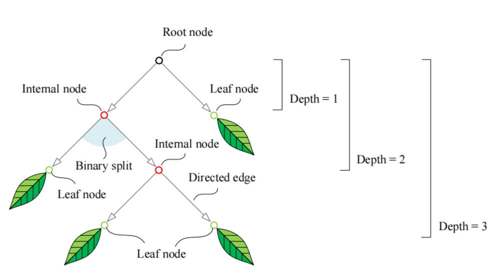
A decision tree is a graphical tool used for decision-making and prediction. It splits the data into smaller parts through a series of choices, ultimately forming a tree-like structure where each node represents a feature, each edge represents a feature’s value, and each leaf node represents the final decision or predicted output.

Basic Components of a Decision Tree

• Root Node: The top node of the tree that represents the overall characteristics of the dataset.

• Internal Nodes: Each internal node represents a feature, which divides the data into different subsets based on the feature’s value.

• Leaf Nodes: The terminal nodes of the tree, representing the final prediction or outcome.

Visualization of a Decision Tree

Below is a simple example of a decision tree:

In this example, the root node is the "Humidity" feature, and the branches further split based on the "Wind Speed" and "Temperature" features.

Building a Decision Tree

The process of building a decision tree generally involves the following steps:

1. Feature Selection
   Choose the optimal feature for the current node. Common feature selection criteria include:

• Information Gain: Measures the reduction in uncertainty after dividing the data based on a feature. The higher the information gain, the more important the feature.

• Gini Impurity: Measures the impurity of the dataset, often used in classification tasks. The lower the Gini impurity, the better the classification.

• Mean Squared Error (MSE): Used for regression tasks, measuring the difference between predicted and actual values.

2. Dataset Splitting
   Split the dataset based on the selected feature and its values. Each split divides the dataset into several subsets, each corresponding to a feature value.

3. Recursive Tree Construction
   Recursively apply feature selection and splitting to each subset until a stopping condition is met, such as:

• The tree reaches its maximum depth.

• The number of samples in the current node is below a certain threshold.

• All samples belong to the same category.

4. Pruning
   To avoid overfitting, the tree may undergo pruning. Pruning refers to removing unnecessary branches from the tree after it is built, simplifying the model. Common pruning methods include:

• Pre-pruning: Check in real-time during the construction if further splits should be made.

• Post-pruning: First, build the full tree and then remove branches from the bottom up.

Pros and Cons of Decision Trees

Advantages:

• Easy to Understand and Interpret: The simple structure of decision trees makes it easy to explain the decision process to non-experts.

• Handles Non-linear Relationships: Can capture complex non-linear relationships in the data.

• No Need for Feature Scaling: Unlike other algorithms, decision trees do not assume a specific distribution of the data, so normalization or standardization is not necessary.

• Suitable for Mixed Data Types: Can handle both numerical and categorical data.

Disadvantages:

• Overfitting: Decision trees are prone to overfitting, especially when the data is sparse or noisy.

• Instability: Small changes in the training data can result in significant changes in the tree structure.

• Bias Toward Multi-valued Features: Decision trees may prefer features with more values, which can affect model performance.

Implementation of Decision Tree

Let’s implement a simple decision tree classifier using Python, demonstrating it with the famous Iris dataset.

1. Data Preparation
   First, ensure the necessary libraries are installed. If scikit-learn and pandas are not installed, run the following command:

   pip install pandas scikit-learn matplotlib seaborn

   Then, we can load the Iris dataset using the following code:

   import pandas as pd
   from sklearn.datasets import load_iris
   
   # Load the dataset
   iris = load_iris()
   data = pd.DataFrame(data=iris.data, columns=iris.feature_names)
   data['target'] = iris.target
   
   # Display the first few rows of the data
   print(data.head())

2. Data Preprocessing
   The Iris dataset is already cleaned, so we will directly use it for model training and testing. Next, we split the dataset into training and testing sets.

   from sklearn.model_selection import train_test_split
   
   # Split the dataset
   X = data.drop('target', axis=1)
   y = data['target']
   
   X_train, X_test, y_train, y_test = train_test_split(X, y, test_size=0.2, random_state=42)
   
   print(f'Training set size: {X_train.shape[0]}, Test set size: {X_test.shape[0]}')

3. Building the Decision Tree Model
   Use the DecisionTreeClassifier from scikit-learn to build the model:

   from sklearn.tree import DecisionTreeClassifier
   
   # Create the decision tree classifier
   clf = DecisionTreeClassifier(random_state=42)
   
   # Train the model
   clf.fit(X_train, y_train)

4. Model Evaluation
   Evaluate the model using the test set and calculate the accuracy:

   from sklearn.metrics import accuracy_score
   
   # Make predictions
   y_pred = clf.predict(X_test)
   
   # Calculate accuracy
   accuracy = accuracy_score(y_test, y_pred)
   print(f'Accuracy: {accuracy:.2f}')

5. Visualizing the Decision Tree
   Scikit-learn provides a simple way to visualize the decision tree:

   from sklearn.tree import plot_tree
   import matplotlib.pyplot as plt
   
   # Plot the decision tree
   plt.figure(figsize=(12, 8))
   plot_tree(clf, filled=True, feature_names=iris.feature_names, class_names=iris.target_names)
   plt.title("Decision Tree for Iris Dataset")
   plt.show()

Pruning the Decision Tree

To avoid overfitting, we can use pruning when constructing the model. The DecisionTreeClassifier in scikit-learn provides parameters to control the tree’s depth and the minimum number of samples required at each node.

# Create the decision tree classifier with maximum depth
clf_pruned = DecisionTreeClassifier(max_depth=3, random_state=42)

# Train the model
clf_pruned.fit(X_train, y_train)

# Make predictions
y_pred_pruned = clf_pruned.predict(X_test)

# Calculate accuracy
accuracy_pruned = accuracy_score(y_test, y_pred_pruned)
print(f'Accuracy of pruned tree: {accuracy_pruned:.2f}')

# Plot the pruned decision tree
plt.figure(figsize=(12, 8))
plot_tree(clf_pruned, filled=True, feature_names=iris.feature_names, class_names=iris.target_names)
plt.title("Pruned Decision Tree for Iris Dataset")
plt.show()

Hyperparameter Tuning for Decision Trees

In practical applications, the performance of decision trees can be further enhanced by tuning hyperparameters. Below are some commonly used hyperparameters and their descriptions:

• max_depth: Controls the maximum depth of the tree to limit its complexity.

• min_samples_split: Specifies the minimum number of samples required to split an internal node.

• min_samples_leaf: Specifies the minimum number of samples required to be present in a leaf node.

• max_features: Limits the maximum number of features considered for each split.

We can use GridSearchCV to optimize hyperparameters:

from sklearn.model_selection import GridSearchCV

# Set the parameter grid
param_grid = {
    'max_depth': [None, 2, 3, 4, 5, 6, 7, 8],
    'min_samples_split': [2, 5, 10],
    'min_samples_leaf': [1, 2, 4]
}

# Create the grid search object
grid_search = GridSearchCV(DecisionTreeClassifier(random_state=42), param_grid, cv=5)

# Perform grid search
grid_search.fit(X_train, y_train)

# Output the best parameters
print("Best parameters:", grid_search.best_params_)

# Train the model with the best parameters
best_clf = grid_search.best_estimator_
y_pred_best = best_clf.predict(X_test)
accuracy_best = accuracy_score(y_test, y_pred_best)
print(f'Accuracy of the best model: {accuracy_best:.2f}')

Real-world Applications of Decision Trees

Decision trees are widely used across various fields. Here are some specific application scenarios:

1. Healthcare
   In medical diagnostics, decision trees assist doctors in predicting diseases based on patients’ symptoms and test results. For instance, a decision tree can help determine if a patient is likely to have diabetes, heart disease, or other conditions by analyzing features like blood sugar, blood pressure, and cholesterol levels, enabling more accurate diagnoses.

2. Finance
   In the financial industry, decision trees are commonly used for credit scoring and risk assessment. Banks can build decision tree models based on applicants’ financial profiles and credit histories to evaluate loan risks. Additionally, decision trees help detect credit card fraud by identifying anomalous transactions.

3. Marketing
   By analyzing consumer behavior data, decision trees assist businesses in customer segmentation. Using information like purchase history and interests, companies can create more targeted marketing strategies. For example, decision trees help identify high-value customers, allowing businesses to offer personalized services and discounts.

4. Manufacturing and Quality Control
   In manufacturing, decision trees analyze product quality data to identify potential causes of defects. By examining production features, businesses can optimize processes and improve product quality. For instance, manufacturers can use decision trees to study the impact of different production conditions on defect rates, aiding in quality control.

5. E-commerce
   On e-commerce platforms, decision trees are utilized in recommendation systems. By analyzing users’ purchase histories and browsing behavior, decision trees recommend products users might find interesting. For example, based on past purchases, a decision tree can infer user preferences and suggest related items.

Future Outlook

With the exponential growth of data and advancements in computational power, decision trees are expected to continue evolving. While decision trees perform well in many applications, they have limitations. For handling large-scale, high-dimensional datasets, single decision trees may underperform. Hence, ensemble methods like Random Forests and Gradient Boosting Trees are becoming preferred alternatives.

Conclusion

As an intuitive and easy-to-implement machine learning model, decision trees are favored for their excellent interpretability and extensive applications. Despite challenges such as overfitting and instability, decision trees can deliver outstanding performance in various real-world scenarios with proper pruning and parameter tuning.

In this article, we provided a detailed overview of the fundamental principles, construction process, and applications of decision trees, supplemented with Python code examples to demonstrate how to use decision trees for classification tasks. We hope this blog helps you gain a better understanding of decision trees and their applications in machine learning.